The Watt Studio

The Internal Rate of Return (IRR) is a powerful financial metric used to assess the profitability of an investment or project. In this 3-part series, we delve into the world of IRR by examining a real-world case study: a Solar + Battery Storage project in the radiant Atacama desert of Chile. While IRR simplifies complex financial transactions, it remains a vital tool for evaluating project feasibility in various industries.

Part 1: Modeling Solar Energy Generation In the first installment, we model the DC and AC energies generated by a solar power plant with a DC/AC ratio of 1.25.

Part 2: Understanding Project Costs and Cashflow The second part delves into the critical components of our project, including CAPEX (Capital Expenditure), OPEX (Operational Expenditure), and cashflow generated from energy sales. We also touch on the concept of EBITDA.

Part 3: Visualizing IRR for Decision-Making In the third and final segment, we evaluate and plot a parametric IRR graph based on energy sales during the day and night. This graphical representation aids in decision-making regarding project financing and initiation.

Our choice of Chile as our project location is strategic. The Ministry of Energy in Chile has generously provided comprehensive weather data, including TMY (Typical Meteorological Year) and historical values, to facilitate renewable energy investments. Additionally, the Atacama desert boasts some of the highest irradiation levels on Earth.

Making Sense of the IRR

Before diving into the details, let’s briefly clarify what IRR means in simple terms. Imagine you’re embarking on a project that requires financing. You secure some funds from sponsors (equity) but often need additional capital (debt) from lenders. After the project’s construction and operation begin, you’re obligated to repay your sponsors and lenders through various means, such as payments, dividends, revenues, and interest. The Cost of Capital represents the rate at which your project breaks even. If the IRR exceeds this rate, the project turns a profit; if it falls short, it’s losing money. The extent to which IRR surpasses the Cost of Capital determines the project’s profitability.

Modeling DC and AC Energy Injection Profiles

We employ the System Advisory Model (SAM) from the National Renewable Energy Laboratory (NREL) to simulate solar PV project conditions accurately. The weather data utilized is a TMY P50 dataseries, sourced from the Ministry-backed initiative (https://solar.minenergia.cl/inicio). For a refresher about P50 weather dataseries, check out my other post over here.

Simulation Parameters:

• Project DC Capacity: 11.25 MWp
• Project AC Capacity: 9.0 MWp
• DC/AC Ratio: 1.25
• Module Capacity: 545W bifacial module
• Module Type: Standard Mono half-cut 144 cells
• Inverter Type: Central inverters with a 3MVA capacity
• BESS System Capacity: 2.75 MWh per unit
• Storage Duration: 6 hours
• BESS Charging Efficiency: 96%
• BESS Discharging Efficiency: 97%
• BESS Life: 15 years
• System Lifetime: 30 years
• BESS Degradation: Linear, approximately 1.5% per year
• BESS Depth of Discharge: 100%
• BESS System Scheme: DC-coupled system
• Charge/Discharge Scheme: Load-shift scheme (charging during the day and discharging at night)

Other Assumptions:

• System Unavailability: Constant 2% applied on the DC side
• Ground Cover Ratio (GCR): 40%
• Soiling: 2%
• Weather File Uncertainty Buffer: Constant 2.5% applied on the DC side

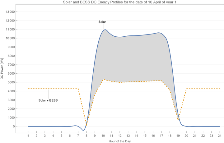
As mentioned before, we are going to use SAM to obtain the DC output at the system (just before going into the batteries/inverters). Once we do that, we are going to perform numerical operations on every hour and day for each year to redistribute the energy throughout each day (charge during the day and discharge during the night). Once done, the generation graph will look something like this (below is a sample day). The blue graph is the original solar DC generation profile, and the orange graph is the adjusted DC generation distributed between the solar and BESS systems. The gray area is how much DC energy was produced during the day, charged in the BESS, and redistributed to be injected at night.

We will then apply the following AC conversion and losses to reach the final injection profiles:

• Inverter efficiency: 98.5%
• Transformer losses: 1%
• AC wiring losses: 1.5%

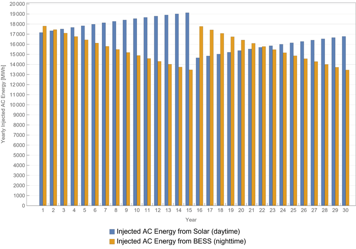
Once we do that and we sum the total energy generated per year, we end up with 2 arrays, one with the energy injected into the grid coming directly from solar, and another one with energy injected into the grid coming from the BESS. We note again that the system lifetime is assumed to be 30 years (will also be the same for the PPA contract duration). Below is a graph showing the energy values per year. Blue is for Solar and Orange is for BESS.

A couple of comments about the injection behavior of the system:

1- After year 15, we are replenishing the BESS system after it’s 15year lifetime ends; once the system reaches 70% efficiency, we will add batteries in order to upgrade the system back to its original 100% efficiency. That element is clear in the graph where, after 15 years of efficiency degradation, energy injection from the BESS system jumps back up to higher values.

2- Even though the solar system and solar panels are degrading at 0.5% per year, the graph shows that the energy injected form the solar system per year is increasing every year instead of decreasing! That is because the BESS system is degrading in parallel at a faster rate (around 1.5% per year), which means more energy will be allocated to the solar total per year than the BESS total. Pretty interesting behavior.

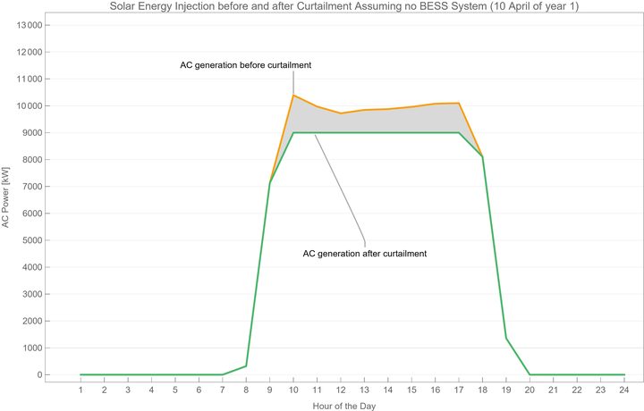
3- During the first year, the specific yield for the system Solar+BESS is equal to 3,100 MWh/MWp. That number would have been around 2,800 MWh/MWp if the system had no BESS integrated to it. The addition of the BESS makes use of 10%+ more energy since less energy would be curtailed during the day at the point of interconnection due to the system MWac limit (see graph below for example day, all the gray area is lost energy due to curtailment at 9MWac at the point of interconnection).

With our generation values established, we can now estimate our cashflow. In Part 2, we’ll explore CAPEX, OPEX, and cashflow cost to gain a deeper understanding of how these elements define the system.

Stay tuned for the next installment in our series, where we’ll unravel other modelling intricacies of this Solar + Battery Storage project in Chile!